另一個使用加速計與低解析度編碼器的位置估測法則 A method for estimating position with accelerometer and low resolution encoders

以下的方法，可以和 Kojima 先生的做法比較 The following method could be compared with the one proposed by Kojima san.

假設位置資料是 $x_1$，速度資料是 $x_2$，加速度資料是 $a$。那麼以狀態空間的方式來描述的話，就會是以下形式 Assume that $x_1$, $x_2$, and $a$ stand for position, velocity, and acceleration, respectively.  The following state equation describes their relationship.

$\left[ \begin{matrix} \dot{x_1} \\ \dot{x_2} \end{matrix} \right]=\left[ \begin{matrix} 0 & 1 \\ 0 & 0 \end{matrix} \right]\left[ \begin{matrix} x_1 \\ x_2 \end{matrix} \right] + \left[ \begin{matrix} 0 \\ 1 \end{matrix} \right] a$

如果位置資料的估測值是 $\hat{x}_1$，速度資料的估測值是 $\hat{x}_2$。那麼以下的狀態空間動態方程式，就可以用來估測位置資料，並且具備較高的解析度。這是利用 Luenberger observer 的概念來做的。Assume that $\hat{x}_1$, and $\hat{x}_2$, stand for position, and velocity estimations, respectively.  The following dynamic equation derived from the idea of state observer could be used to estimate the position and velocity signals with better resolution and accuracy.

$\frac{d}{dt} \left[ \begin{matrix} \hat{x}_1 \\ \hat{x}_2 \end{matrix} \right]=\left[ \begin{matrix} 0 & 1 \\ 0 & 0 \end{matrix} \right]\left[ \begin{matrix} \hat{x}_1 \\ \hat{x}_2 \end{matrix} \right] + \left[ \begin{matrix} 0 \\ 1 \end{matrix} \right] a + \left[ \begin{matrix} g_1 \\ g_2 \end{matrix} \right] (x_1 - \hat{x}_1)$

$g_1$ 與 $g_2$ 的設計可以用 $g_1=2\zeta \omega_n$，$g_2=\omega_n^2$，來設計，$\zeta$ 是 damping ratio ，$\omega_n$ 可以看成頻寬，$\zeta$ 可以選擇 [0.7, 1] 的範圍。Gains of $g_1$ and $g_2$ can be adjusted by using second order systems.

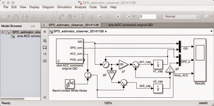
以下就是假設編碼器的解析度是 16 pulses/r 的模擬結果。其中加速度的資料來自加速規，而且我加了一些雜訊已接近真實情況。目前看起來還不錯。接下來就是數位化的工作。The following SIMULINK behavior model assumes that the resolution of a encoder is 16 pulses/r, and acceleration signal is added some white noise.

當我把編碼器輸出信號的單位弄錯時，下圖是錯誤的模擬結果，速度信號不對。The following incorrect results come from the wrong setting of the unit of position signals.  The estimated velocity signal does not match the true one.

修正過後的結果，可以看出位置與速度都正確的跟上了。The followings are correct results.

放大來看，可以看出位置信號的解析度的確增加了，加速規雜訊的影響也不大。

整個估測器的 SIMULINK 行為模型。

產生模擬信號的SIMULINK 行為模型。

離散時間的模擬看起來也可以了，取樣時間設定為 $T_s$ = 1ms, Discrete time simulations with $T_s$ = 1ms seems OK now.

一個電腦鼠運與自走車運動控制的新方法 A new method for the motion control of micromouse and robotracers

為了解決因編碼器解析度帶來差分的雜訊問題，我做了一個二階的位置與速度估測器，並且用這一些估測值來控制電腦鼠運與自走車的位置與速度。
A second order filter is devised in this article to estimate the position and velocity of wheeled mobile robots such that the noise effect arose from difference methods can be lessened.

我在 MPLAB 中利用以下的副程式實現了這樣一個演算法 The algorithm is implemented in the MPLAB environment

//--------- Functions -----------------------------------------
// Function Name : EST_FILTER
// Description   : 2nd order filter for vc and w
// input              : struct ESTIMATOR_S est_ps, or est_ths
// output            : struct ESTIMATOR_S est_ps, or est_ths
//-------------------------------------------------------------
struct ESTIMATOR_S EST_FILTER(struct ESTIMATOR_S states, long ref)
{
//long er_estp2;

states.yv.n = states.yv.n1 + states.erv.n1;
states.yp.n = states.yp.n1 + states.yv.n1;
states.er = ref - states.yp.n;
states.erv.n = (states.er>>2) - states.yv.n;
states.erv.n1 = states.erv.n;
states.yv.n1 = states.yv.n;
states.yp.n1 = states.yp.n;

return (states);
}

struct ESTIMATOR_S { union POSITION yp; struct FILTER_S yv; struct FILTER_S erv; long er; };

struct FILTER_S { int n; int n1; };

union POSITION { struct { long n; // in pulses, 81 pulses ~ 1mm, Q26.5 long n1; }; struct { unsigned int Ln; unsigned int Hn; unsigned int Ln1; unsigned int Hn1; }; } ;

其中 ref 代表真實的編碼器位置信號，states.yp.n 與 states.yp.n1 分別表示現在與過去一個取樣時間的編碼器位置信號估測值，states.yv.n 與 states.yv.n1 分別表示現在與過去一個取樣時間的編碼器速度信號估測值，states.er 是編碼器位置信號真實值與估測值之間的誤差。

states.erv.n = (states.er>>2) - states.yv.n;

上述方程式中的 states.erv.n 是使用編碼器位置信號真實值與估測值之間的誤差乘以 P 增益 0.25，加上編碼器速度信號估測值乘以 D 增益 1的結果，然後再積分得到編碼器速度信號估測值。

states.yv.n = states.yv.n1 + states.erv.n1; $\leftarrow y_v[n] = y_v[n-1] + erv[n-1]*T_s$

真正執行程式時，為了提高解析度，我將編碼器位置信號真實值放大 32 倍。

est_psR = EST_FILTER(est_psR, (out_pR.n<<5));
est_psL = EST_FILTER(est_psL, (out_pL.n<<5));

做位置控制的程式段

// find feedback variables
POS_con.pQEI = ((est_psR.yp.n + est_psL.yp.n)>>1);
ANG_con.pQEI = (est_psR.yp.n - est_psL.yp.n);

// find controlled errors
POS_con.perr = POS_con.pcom - POS_con.pQEI;
ANG_con.perr = ANG_con.pcom - ANG_con.pQEI;

// find motor command ->  $K_pe_p - K_v v_c^e$, and $K_p\theta_p - K_v \omega_c^e$
POS_PWM = (POS_con.perr>>1) - 9*((est_psL.yv.n+est_psR.yv.n)>>1);
ANG_PWM = (ANG_con.perr>>2) - 4*(est_psR.yv.n-est_psL.yv.n);

// find right and left motor commands
R_PWM = POS_PWM + ANG_PWM;
if (R_PWM>PWM_100) R_PWM = PWM_100;
else if (R_PWM<-PWM_100) R_PWM = -PWM_100;
//
L_PWM = POS_PWM - ANG_PWM;
if (L_PWM>PWM_100) L_PWM = PWM_100;
else if (L_PWM<-PWM_100) L_PWM = -PWM_100;

實驗結果 Experimental results for center and angular velocity

二次曲線內差法 Second order interpolation algorithm

假設我們有以下三組資料 assume that we have the following 3 pairs of data,
$(x_1-\Delta, y_0)$, $(x_1, y_1)$, and $(x_1+\Delta, y_2)$

利用一個一元二次方程式來表示通過這三個點的曲線，參數為 $a, b, c$
A second order equation is used to represent a curve that passes these 3 points

$y_0 = a(x_1-\Delta)^2 + b(x_1-\Delta) + c$
$y_1 = ax_1^2 + bx_1 + c$
$y_2 = a(x_1+\Delta)^2 + b(x_1+\Delta) + c$

以下討論如何利用這三個點以及內差法，來找出當 $x=x_1+\alpha\Delta$ 的 y 值
The following discussion is used to predict what the $y$ value is, when $x=x_1+\alpha\Delta$

由於 Since

$y_0 = a(x_1-\Delta)^2 + b(x_1-\Delta) + c = y_1 - 2a\Delta x_1 + a\Delta^2 - b\Delta$
$y_2 = a(x_1+\Delta)^2 + b(x_1+\Delta) + c = y_1 + 2a\Delta x_1 + a\Delta^2 + b\Delta$

因此 Therefore

$y = a(x_1+\alpha\Delta)^2 + b(x_1+\alpha\Delta) + c = y_1 + \alpha(y_2-y_1) - \alpha(1-\alpha)a\Delta^2$

至於變數 $a$，可以利用以下關係求出來
and the variable $a$ can be found by using the following equation

$a = \frac{y_0+y_2-2y_1}{2\Delta^2}$

只是計算時，可以考慮使用 $a\Delta^2$，
It would be easier in calculation if we use the following equation

$a\Delta^2 = 0.5(y_0+y_2-2y_1)$

也就是說

$y = y_1 + \alpha(y_2-y_1) - 0.5\alpha(1-\alpha)(y_0+y_2-2y_1)$

其中的 $y_1 + \alpha(y_2-y_1)$，就是線性內差的結果，而 $- 0.5\alpha(1-\alpha)(y_0+y_2-2y_1)$ 可以看成是二次內差法針對一次內差法的修正項。

但也有可能我們必須求出當 $x=x_1-\Delta + \alpha\Delta$ 的 y 值，也就是自變數 $x$ 的值落在建表自變數的第一個與第二個之間的數值 It may be possible that we have to find the interpolation value that corresponds to $x=x_1-\Delta + \alpha\Delta$.  This would occur when the $x$ value lies in the interval between the first and the second $x$ value of the table.

$y = a(x_1-\Delta+\alpha\Delta)^2 + b(x_1-\Delta+\alpha\Delta) + c = y_0 + (1-\alpha)(y_1-y_0) - \alpha(1-\alpha)a\Delta^2$

可以看出修正項是一樣的。

陀螺儀與編碼器濾波後信號的比較 (Comparisons of gyro and filtered encoder signals)

爲了能夠得到比較乾淨的「車頭角速度」估測，我需要一個乾淨的「車中心角速度」。
To get a clean estimate of 'head angular velocity' (The place where my Beetle robotracer is controlled to follow the line), I need a clean body angular velocity.

基於使用 PD 控制來調整循跡時的角速度，我試了兩個方法，一個是用編碼器濾波後的兩輪速度信號相減 (右輪減左輪)，另一個是使用陀螺儀。
Based on PD control algorithm to adjust the angular velocity command to follow the line, I tried two methods to obtain the body angular velocity.  The first one is to use filtered encoder signals (right wheel velocity - left wheel velocity), and the other one is to use gyro signals.

可惜這兩個信號都不夠乾淨，以下是實驗結果。
It is a pity that both methods are not good enough, and the experimental results are shown in the following figure.

恐怕我得試試「基於誤差大小的變動比例增益」控制方法來循跡了。
I am afraid that I have to use gain scheduled proportional control based on the line following error to reach my goal.

一個簡單提升解析度的速度估測法則 A simple velocity estimation method for micromouse

在電腦鼠的製作過程中，運動控制是很重要的一個部分。
Motion control is a very important part for a micromouse.

以下是一個利用兩個積分器，速度回授，以及位置控制做出來的一個簡單提升解析度的速度估測法則(與傳統差分法的比較)。
The following is a simple but effective velocity estimation method with 2 integrators, velocity feedback, and position control for micormouse to increase resolution beyond difference traditional difference method.

以下圖形中，是拿編碼器所提供的整數形態位置脈波數作為伺服控制中的命令，然後取出以回授估測位置為輸出的積分器之輸入信號作為速度的估測值與傳統差分法的比較。
The following figure show the comparison of the proposed method and the traditional difference method for velocity estimation by using position values obtained from encoders as an input command for a servo control loop.  The input signal of an integrator whose output is used as estimated position values is treated as the estimated velocity.

上面的兩個圖形，是直接使用編碼器所提供的整數形態位置脈波數作為伺服控制中的命令的結果，而下面的兩個圖形，則是先將編碼器所提供的整數形態位置脈波數放大8倍後，再作為伺服控制中的命令的結果。
The top 2 plots show the results of no scaling of encoder inputs, which means no fractional part is kept in the calculation when implementing the algorithm.  The lower plots shows the results of using 3 digits to represent the fractional part during calculation.

可以看出保留小數部分，可以得到更好的結果。
It is clearly seen the superiority of the results which kept fractional part during calculation.

A few thoughts about the normalization of IR sensor outputs

I found some interesting things when I tried to determine what the best resistor values were for limiting the current flowing through the infrared LEDs.

1. If I assume that the light emitted from the IR LED is of cone shape in 3D, then the projection on the ground would mostly in our case be an ellipse.
2. The long axis of the ellipse that created by the center LED sits on the moving direction of my Robotracer, Beetle.
3. It is observed that when I try to move my Robotracer to cross the line and record the sensor readings along the way, there would be a small part of the sensor readings that seems not changed (see Figure 1).  The reason for this observation can be illustrated by using Figure 2.
4. Therefore, the maximum of the sensor readings when crossing the line would be smaller than that when the robotracer is running.  This, I think, makes my line position estimation (weighted average) give error results at some point, not always.  I seem to solve this problem by lowering the normalized sensor output range, from [50, 900] to [50, 750], and by purposely making the maximum values of those raw IR sensor readings larger (multiplied by 1.3).  This deserves more investigation.  I came up with this solution because I thought when the robotracer try to correct the sensor readings with the normalization parameters I got from moving the robotracer to cross the line, may make the reading corrections exceeds the variable type limit (I use unsigned int for sensor readings).  A second thought on this problem shows the guess may not be true.

Fig.1 Sensor readings of the Robotracer, Beetle, when crossing the line

Fig. 2.  The projections of the IR LEDs on the ground of the Robotracer, Beetle.  (left) when the robotracer is running, and (right) when it records the sensor outputs for normalization

Robotracer Beetle: Normalization of infrared sensor outputs

This is my robotracer, Beetle, and I have almost finished checking its capabilities.  The only thing left is to write data to the flash memory of the microcontroller, dsPICmc806.

The followings are experimental results for its normalization of infrared (IR) sensor outputs.  The data of 7 IR sensor outputs is obtained when I push Beetle to cross a horizontal white line.

The first figure shows the results when the ground material is similar to that used in Taiwan's contest.

Currently, I have no idea about why the shape of the sensor outputs do not look like bell.  Is it because the angle between the emitting line of IR LEDs and the ground is about 60 degrees? This makes the projection of the light on the ground similar to the shape of a rain drop (according to theory, the shape should be an ellipse if the light emitted from IR LEDs are cones).

The following figure shows the theoretical prediction of the projection of my LEDs on the ground. (I write a MATLAB program to produce the figure)

All the maximum and minimum values of the sensor outputs are mapped using a linear function to 900 and 50, which is shown at the bottom half of the figure.

The mapping function is

$y = y_{min} + (y_{max} - y_{min})/(x_{max} - x_{min})(x - x_{min})$

The following are the results when I used a printed track on a poster, and the reflection ratio is larger than that of the contest ground.

03/20/2014

The previous experimental results seem to suffer residual voltage problem (D2 is the most obvious one), because I did not wait some time to let the residual voltage from the other LED reflected light dies out, and sample immediately after the previous sampling process ends.  The followings are revised version for both poster and contest ground normalization.

From tomorrow on, I will try to find out the impact of the differences on the estimation of the position of line tracks.

Kato 與我關於電腦鼠角速度曲線平滑化的討論 Discussions of speed command profiles for micromouse to make turns

這一篇文章主要是要討論 Kato 先生關於電腦鼠轉彎過程角加速度曲線的想法。

http://blog.livedoor.jp/robolabo/archives/51500936.html

\( \omega = \frac{1}{2} \left(1-\cos \left( \pi \frac{t(2.5-t)}{1.5} \right) \right), t \in [0, 1] \)

取微分得到角加速度

$\frac{d \omega}{dt}=\sin(\pi t(2.5-t)/1.5) \frac{\pi (2.5-2t)}{3}$

但看起來，角加速度的極大值並不容易有解析解可以求得。試試看找出角加速度的微分

\( \frac{d^2 \omega}{dt^2} = \cos \left( \pi \frac{t(2.5-t)}{1.5} \right) \frac{\pi^2(2.5-2t)^2}{4.5} - \frac{2\pi}{3} \sin \left( \pi \frac{t(2.5-t)}{1.5} \right) \)

可以看出即使令角加速度的微分為零，也不容易找出 $t$ 的解，進而找到角加速度的極大值。

找角加速度極大值的原因是希望能限制它的大小，以免造成電腦鼠在轉彎時的滑動。

事實上，Kato 的做法可以用以下的參數化方程式來討論，端看使用者喜歡哪一個

\( \omega(t)=\frac{1}{2} \left( 1-\cos \left(\pi t \frac{\gamma-t}{\gamma-1}\right)  \right),  \gamma \ge 2 \)

以下是與原始餘弦函數與不同的參數 $\gamma$ 值作了比較後的圖形

可以看得出來，$\gamma$ 值越大，曲線越平緩，越接近原始的餘弦函數。

其實這樣的一個做法是靠著調整時間軸 $t$ 由 0 到 1 的變動速度來達成，以平方函數來看 $t(\gamma-t)$，在 $t$ 由 0 到 $\gamma/2$ 的變動斜率 $\gamma-2t$，是由大到小。換句話說，第一段角速度的加速過程，也就是餘弦函數由 $0$ 到 $\pi/2$ 的這一段，會進行得比較快，而第二段角速度的加速過程，也就是餘弦函數由 $pi/2$ 到 $\pi$ 的這一段，則會相對進行得比較慢。但這樣的趨勢，會隨著 $\gamma$ 越大而越不明顯。

以這樣的想法來看，其實並不一定要平方函數，根號函數亦可。例如

\( \omega(t)=\frac{1}{2} \left( 1-\cos \left(\pi t^\gamma\right)  \right),  0.5 < \gamma < 1 \)

以下就是 $\gamma = 0.7, 0.8, 0.9$ 以及 Kato 做法的比較。

我的做法

另一個做法是分段使用餘弦函數，以 $\sigma$ 作為控制變數，$\sigma >1$，用來調整第一段緩加速的時間。

原始餘弦函數若是

\( \omega_o(t) = 0.5\alpha(1-\cos (\beta \pi t))，t \in [0, 1/\beta] \)，

其中角加速度的極大值由以下的微分運算可以知道為 $0.5\alpha \beta \pi$

\( \frac{d\omega_o(t)}{dt} = 0.5\alpha \beta \pi \sin(\beta \pi t), t \in [0, 1/\beta] \)

把原始餘弦函數在 $t=0.5/\beta$ 的點，以及其對應的角加速度大小作為「控制點」，將它移動到 $t=0.5/(\sigma \beta)$ 的點。因此，為了保持角加速度的極大值為 $0.5\alpha \beta \pi$，就將第一段角速度曲線的緩加速定義成

\( \omega_1(t) = \frac{0.5\alpha}{\sigma}(1-\cos (\sigma \beta \pi t)),   t \in \left[ 0, \frac{0.5}{\beta \sigma} \right] \)。

至於第二段角速度曲線 $\omega_2(t)$ 的變化過程，必須符合以下三個條件

1. $\omega_1\left( \frac{0.5}{\beta \sigma} \right) = \omega_2\left( \frac{0.5}{\beta \sigma} \right) $
2. $\omega_2 \left( \frac{1}{\beta} \right) = \alpha$。
3. $\frac{d\omega_1}{dt}\left(\frac{0.5}{\beta \sigma}\right) = \frac{d\omega_2}{dt}\left(\frac{0.5}{\beta \sigma}\right)$

假設

\( \omega_2(t) = a(b-c\cos(dt+e)) \)。

那麼

\( d\frac{0.5}{\beta \sigma}+e=\frac{\pi}{2}, d\frac{1}{\beta}+e=\pi \)。

因此

\( d \left( \frac{1}{\beta} - \frac{1}{2\beta\sigma} \right) = \frac{\pi}{2} \rightarrow d = \frac{\sigma\beta\pi}{2\sigma-1}, e = \pi-\frac{d}{\beta} = \frac{(\sigma-1)\pi}{2\sigma-1} \)

當 $dt_1+e = 0.5\pi$ 時，

\( \omega_2(t_1) = ab = \frac{\alpha}{2\sigma} \)；

\( \frac{d\omega_2}{dt}(t_1) = 0.5\alpha\beta\pi = acd\sin(dt_1+e) = acd \)

由於 $d$ 已經找出大小了，所以

\( acd = 0.5\alpha\beta\pi \rightarrow ac = \frac{0.5\alpha\beta\pi}{d} = \frac{(2\sigma-1)\alpha}{2\sigma} \)

當 $ct_2+d = \pi$ 時，

\( \omega_2(t_2) = a(b+c) = \alpha \)；

剩下三個未知數 $a, b, c$，但上面三個方程式卻是相依，因為

\( ab = \frac{\alpha}{2\sigma}, ac = \frac{(2\sigma-1)\alpha}{2\sigma} \rightarrow a(b+c) = \alpha \)。

因此，令 $c=1$，則

\( a = \alpha\frac{2\sigma-1}{2\sigma}, b = \frac{\alpha}{2a\sigma} = \frac{1}{2\sigma-1} \)。

以下就是完整的角速度曲線公式

\( f(t) = \left\{ \begin{array}{1,1} \frac{\alpha}{2\sigma} [1-\cos (\sigma \beta \pi t)] & t \in \left[0, \frac{1}{2\sigma \beta} \right) \\ \frac{(2\sigma-1)\alpha}{2\sigma} \left[ \frac{1}{2\sigma-1}-\cos \left( \frac{\sigma\beta\pi}{2\sigma -1}t + \frac{(\sigma-1)\pi}{2\sigma-1} \right) \right] & t \in \left[ \frac{1}{2\sigma \beta}, \frac{1}{\beta} \right] \end{array} \right. \)

接下來應該是要找出角速度曲線加減速過程的累積角度，也就是上述曲線的積分。會有一些複雜，目前記錄在簡報擋上，下次再整理上來。

$ \int_0^{t_1} \omega_1(t) \text{d}t = \int_0^{t_1} \frac{\alpha}{2\sigma} [1-\cos(\sigma\beta\pi t)] = \frac{\alpha}{2\sigma} \frac{1}{2\sigma\beta} - \frac{\alpha}{2\sigma} \frac{1}{\sigma\beta\pi} \sin(\sigma\beta\pi t_1) = \frac{\alpha}{4\sigma^2\beta} - \frac{\alpha}{2\sigma^2\beta\pi}, t_1 = \frac{1}{2\sigma\beta} $

\( \int_{t_1}^{t_2} \omega_2(t) \text{d}t = \frac{\alpha}{2\sigma} (t_2-t_1) - \frac{(2\sigma-1)\alpha}{2\sigma} \frac{2\sigma-1}{\sigma\beta\pi} \left. \sin\left( \frac{\sigma\beta\pi}{2\sigma-1}t + \frac{(\sigma-1)\pi}{2\sigma-1} \right) \right|_{t_1}^{t_2} = \)

但我把模擬程式也寫好了。